Introduction to Macro Economics & Financial Accounting

Investment Under Certainty

Capital Budgeting is the process by which the firm decides which long-term investments to make. Capital Budgeting projects, i.e., potential long-term investments, are expected to generate cash flows over several years.

Capital Budgeting also explains the decisions in which all the incomes and expenditures are covered. These decisions involve all inflows and outflows of funds of an undertaking for a particular period of time.

Capital Budgeting techniques under certainty can be divided into the following two groups −

Non Discounted Cash Flow

• Pay Back Period
• Accounting Rate of Return (ARR)

Discounted Cash Flow

• Net Present Value (NPV)
• Profitability Index (PI)
• Internal Rate of Return (IRR)

The payback period (PBP) is the traditional method of capital budgeting. It is the simplest and perhaps the most widely used quantitative method for appraising capital expenditure decision; i.e. it is the number of years required to recover the original cash outlay invested in a project.

Non-Discounted Cash Flow

Non-discounted cash flow techniques are also known as traditional techniques.

Pay Back Period

Payback period is one of the traditional methods of budgeting. It is widely used as quantitative method and is the simplest method in capital expenditure decision. Payback period helps in analyzing the number of years required to recover the original cash outlay invested in a particular project. The formula widely used to calculate payback period is −

PBP =

Initial InvestmentConstant annual cash inflow

Advantages of Using PBP

PBP is a cost effective and easy to calculate method. It is simple to use and does not require much of the time for calculation. It is more helpful for short term earnings.

Accounting Rate of Return (ARR)

The ARR is the ratio after tax profit divided by the average investment. ARR is also known as return on investment method (ROI). Following formula is usually used to calculate ARR −

ARR =

Average annual profit after taxAverage investment

 ×

100

The average profits after tax are obtained by adding up the profit after tax for each year and dividing the result by the number of years.

Advantages of Using ARR

ARR is simple to use and as it is based on accounting information, it is easily available. ARR is usually used as a performance evaluation measure and not as a decision making tool as it does not use cash flow information.

Discounted Cash Flow Techniques

Discounted cash flow techniques consider time value of money and are therefore also known as modern techniques.

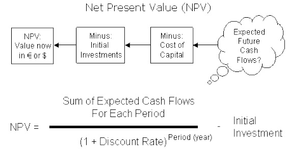
Net Present Value (NPV)

The net present value is one of the discounted cash flow techniques. It is the difference between the present value of future cash inflows and the present value of the initial outlay, discounted at the firm’s cost of capital. It recognizes the cash flow streams at different time intervals and can be computed only when they are expressed in terms of common denominator (present value). Present value is calculated by determining an appropriate discount rate. NPV is calculated with the help of equation.

NPV = Present value of cash inflows − Initial investment.

Advantages

NPV is considered as the most appropriate measure of profitability. It considers all the years of cash flow, and recognizes the time value for money. It is an absolute measure of profitability that means it gives output in terms of absolute amount. The NPVs of the projects can be added together which is not possible in other methods.

Profitability Index (PI)

Profitability index method is also known as benefit cost ratio as numerator measures benefits and denominator measures cost like the NPV approach. It is the ratio obtained by dividing the present value of future cash inflows by the present value of cash outlays. Mathematically it is defined as −

PI =

Present value of cash inflowInitial cash outlay

Advantages

In a capital rationing situation, PI is a better evaluation method as compared to NPV method. It considers the time value of money along cash flows generated by the project.

		Present Cash Value
Year	Cash Flows	@ 5% Discount	@ 10% Discount
0	$ -10,000.00	$ -10,000.00	$ -10,000.00
1	$ 2,000.00	$ 1,905.00	$ 1,818.00
2	$ 2,000.00	$ 1,814.00	$ 1,653.00
3	$ 2,000.00	$ 1,728.00	$ 1,503.00
4	$ 2,000.00	$ 1,645.00	$ 1,366.00
5	$ 5,000.00	$ 3,918.00	$ 3,105.00
	Total	$ 1,010.00	$ -555.00

Profitability Index (5%) =

$11010$10000

 = 1.101

Profitability Index (10%) =

$9445$10000

 = .9445

Internal Rate of Return (IRR)

Internal rate of return is also known as yield on investment. IRR depends entirely on the initial outlay of the projects which are evaluated. It is the compound annual rate of return that the firm earns, if it invests in the project and receives the given cash inflows. Mathematically IRR is determined by the following equation −

IRR = T∑t=1

C_t(1 + r)^t

 − 1c₀

Where,

R = The internal rate of return

C_t = Cash inflows at t period

C₀ = Initial investment

Example −

Internal Rate of Return
Opening Balance	-100,000
Year 1 Cash Flow	110000
Year 2 Cash Flow	113000
Year 3 Cash Flow	117000
Year 4 Cash Flow	120000
Year 5 Cash Flow	122000
Proceeds from Sale	1100000
IRR	9.14%

Advantages

IRR considers the total cash flows generated by a project over the life of the project. It measures profitability of the projects in percentage and can be easily compared with the opportunity cost of capital. It also considers the time value of money.

Circular Flow Model of Economy

Circular flow model is the basic economic model and it describes the flow of money and products throughout the economy in a very simplified manner. This model divides the market into two categories −

• Market of goods and services
• Market for factor of production

The circular flow diagram displays the relationship of resources and money between firms and households. Every adult individual understands its basic structure from personal experience. Firms employ workers, who spend their income on goods produced by the firms. This money is then used to compensate the workers and buy raw materials to make the goods. This is the basic structure behind the circular flow diagram. Let’s have a look at the following diagram −

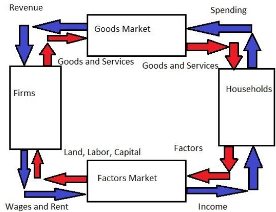
In the above model, we can see that the firms and the households interact with each other in both product market as well as factor of production market. The product market is the market where all the products by the firms are exchanged and factors of production market is where inputs such as land, labor, capital and resources are exchanged. Households sell their resources to the businesses in the factor market to earn money. The prices of the resources, the businesses purchase are “costs”. Business produces goods utilizing the resources provided by the households, which are then sold in the product market. Households use their incomes to purchase these goods in the product market. In return for the goods, businesses bring in revenue.

Inflation

In economics, inflation means rise in the general level of prices of goods and services over a period of time in an economy. Inflation may affect the economy either in positive way or negative way.

Causes of Inflation

The causes of inflation are as follows −

• Inflation may occur sometimes due to excessive bank credit or currency depreciation.
• It may be caused due to increase in demand in relation to supply of all types goods and services due to a rapid increase in population.
• Inflation also may be also be caused by a change in the value of production costs of goods.
• Export boom inflation also comes into existence when a considerable increase in exports may cause a shortage in the home country.

Inflation is also caused by decrease in supplies, consumer confidence, and corporate decisions to charge more.

Measures to Control Inflation

There are many ways of controlling inflation in an economy −

Monetary Measure

The most important method of controlling inflation is monetary policy of the Central Bank. Most central banks use high interest rates as a way to fight inflation. Following are the monetary measures used to control inflation −

• Bank Rate Policy − Bank rate policy is the most common tool against inflation. The increase in bank rate increases the cost of borrowings which reduces commercial banks borrowing from the central bank.
• Cash Reserve Ratio − To control inflation, the central bank needs to raise CRR which helps in reducing the lending capacity of the commercial banks.
• Open Market Operations − Open market operations mean the sale and purchase of government securities and bonds by the central bank.

Fiscal Policy

Fiscal measures are another important set of measures to control inflation which include taxation, public borrowings, and government expenses. Some of the fiscal measures to control inflation are as follows −

• Increase in savings
• Increase in taxes
• Surplus budgets

Wage and Price Controls

Wage and price controls help in controlling wages as the price increases. Price control and wage control is a short term measure but is successful; since in long run, it controls inflation along with rationing.

Impact of Inflation on Managerial Decision Making

Inflation is of course the all too familiar problem of too much money (demand) chasing too few goods (supply), with the upshot of prices and expectations everywhere tending to rise higher and higher.

The Role of a Manager

In these circumstance, a business manager has to take appropriate decisions and measures based on macro economic uncertainties like inflation and the occasional recession.

A true test of a business manager lies in delivering profitability ie., the extent to which he increases revenues and also reduces costs even during economic uncertainties.

In the current scenario, they are supposed to get faster solutions to the problems of coping with soaring prices (for example) by understanding the process of how inflation distorts the traditional functions of money along with recommendations.

The Effect of Management

The bottom-line impact is that, Customers / clients reward efficient management with profits and penalize inefficient management with losses. Hence, it is advisable to be well prepared to tackle these areas.

Market Structure & Pricing Decisions

Price determination is one of the most crucial aspects in economics. Business managers are expected to make perfect decisions based on their knowledge and judgment. Since every economic activity in the market is measured as per price, it is important to know the concepts and theories related to pricing. Pricing discusses the rationale and assumptions behind pricing decisions. It analyzes unique market needs and discusses how business managers reach upon final pricing decisions.

It explains the equilibrium of a firm and is the interaction of the demand faced by the firm and its supply curve. The equilibrium condition differs under perfect competition, monopoly, monopolistic competition, and oligopoly. Time element is of great relevance in the theory of pricing since one of the two determinants of price, namely supply depends on the time allowed to it for adjustment.

Market Structure

A market is the area where buyers and sellers contact each other and exchange goods and services. Market structure is said to be the characteristics of the market. Market structures are basically the number of firms in the market that produce identical goods and services. Market structure influences the behavior of firms to a great extent. The market structure affects the supply of different commodities in the market.

When the competition is high there is a high supply of commodity as different companies try to dominate the markets and it also creates barriers to entry for the companies that intend to join that market. A monopoly market has the biggest level of barriers to entry while the perfectly competitive market has zero percent level of barriers to entry. Firms are more efficient in a competitive market than in a monopoly structure.

Perfect Competition

Perfect competition is a situation prevailing in a market in which buyers and sellers are so numerous and well informed that all elements of monopoly are absent and the market price of a commodity is beyond the control of individual buyers and sellers

With many firms and a homogeneous product under perfect competition no individual firm is in a position to influence the price of the product that means price elasticity of demand for a single firm will be infinite.

Pricing Decisions

Determinants of Price Under Perfect Competition

Market price is determined by the equilibrium between demand and supply in a market period or very short run. The market period is a period in which the maximum that can be supplied is limited by the existing stock. The market period is so short that more cannot be produced in response to increased demand. The firms can sell only what they have already produced. This market period may be an hour, a day or a few days or even a few weeks depending upon the nature of the product.

Market Price of a Perishable Commodity

In the case of perishable commodity like fish, the supply is limited by the available quantity on that day. It cannot be stored for the next market period and therefore the whole of it must be sold away on the same day whatever the price may be.

Market Price of Non-Perishable and Reproducible Goods

In case of non-perishable but reproducible goods, some of the goods can be preserved or kept back from the market and carried over to the next market period. There will then be two critical price levels.

The first, if price is very high the seller will be prepared to sell the whole stock. The second level is set by a low price at which the seller would not sell any amount in the present market period, but will hold back the whole stock for some better time. The price below which the seller will refuse to sell is called the Reserve Price.

Monopolistic Competition

Monopolistic competition is a form of market structure in which a large number of independent firms are supplying products that are slightly differentiated from the point of view of buyers. Thus, the products of the competing firms are close but not perfect substitutes because buyers do not regard them as identical. This situation arises when the same commodity is being sold under different brand names, each brand being slightly different from the others.

For example − Lux, Liril, Dove, etc.

Each firm is therefore the sole producer of a particular brand or “product”. It is monopolist as far as a particular brand is concerned. However, since the various brands are close substitutes, a large number of “monopoly” producers of these brands are involved in a keen competition with one another. This type of market structure, where there is competition among a large number of “monopolists” is called monopolistic competition.

In addition to product differentiation, the other three basic characteristics of monopolistic competition are −

• There are large number of independent sellers and buyers in the market.
• The relative market shares of all sellers are insignificant and more or less equal. That is, seller-concentration in the market is almost non-existent.
• There are neither any legal nor any economic barriers against the entry of new firms into the market. New firms are free to enter the market and existing firms are free to leave the market.
• In other words, product differentiation is the only characteristic that distinguishes monopolistic competition from perfect competition.

Monopoly

Monopoly is said to exist when one firm is the sole producer or seller of a product which has no close substitutes. According to this definition, there must be a single producer or seller of a product. If there are many producers producing a product, either perfect competition or monopolistic competition will prevail depending upon whether the product is homogeneous or differentiated.

On the other hand, when there are few producers, oligopoly is said to exist. A second condition which is essential for a firm to be called monopolist is that no close substitutes for the product of that firm should be available.

From above it follows that for the monopoly to exist, following things are essential −

• One and only one firm produces and sells a particular commodity or a service.
• There are no rivals or direct competitors of the firm.
• No other seller can enter the market for whatever reasons legal, technical, or economic.
• Monopolist is a price maker. He tries to take the best of whatever demand and cost conditions exist without the fear of new firms entering to compete away his profits.

The concept of market power applies to an individual enterprise or to a group of enterprises acting collectively. For the individual firm, it expresses the extent to which the firm has discretion over the price that it charges. The baseline of zero market power is set by the individual firm that produces and sells a homogeneous product alongside many other similar firms that all sell the same product.

Since all of the firms sell the identical product, the individual sellers are not distinctive. Buyers care solely about finding the seller with the lowest price.

In this context of “perfect competition”, all firms sell at an identical price that is equal to their marginal costs and no individual firm possess any market power. If any firm were to raise its price slightly above the market-determined price, it would lose all of its customers and if a firm were to reduce its price slightly below the market price, it would be swamped with customers who switch from the other firms.

Accordingly, the standard definition for market power is to define it as the divergence between price and marginal cost, expressed relative to price. In Mathematical terms we may define it as −

L = 

(P − MC)P

Oligopoly

In an oligopolistic market there are small number of firms so that sellers are conscious of their interdependence. The competition is not perfect, yet the rivalry among firms is high. Given that there are large number of possible reactions of competitors, the behavior of firms may assume various forms. Thus there are various models of oligopolistic behavior, each based on different reactions patterns of rivals.

Oligopoly is a situation in which only a few firms are competing in the market for a particular commodity. The distinguishing characteristics of oligopoly are such that neither the theory of monopolistic competition nor the theory of monopoly can explain the behavior of an oligopolistic firm.

Two of the main characteristics of Oligopoly are briefly explained below −

• Under oligopoly the number of competing firms being small, each firm controls an important proportion of the total supply. Consequently, the effect of a change in the price or output of one firm upon the sales of its rival firms is noticeable and not insignificant. When any firm takes an action its rivals will in all probability react to it. The behavior of oligopolistic firms is interdependent and not independent or atomistic as is the case under perfect or monopolistic competition.
• Under oligopoly new entry is difficult. It is neither free nor barred. Hence the condition of entry becomes an important factor determining the price or output decisions of oligopolistic firms and preventing or limiting entry of an important objective.

For Example − Aircraft manufacturing, in some countries: wireless communication, media, and banking.

Pricing Strategies

Pricing is the process of determining what a company will receive in exchange for its product or service. A business can use a variety of pricing strategies when selling a product or service. The price can be set to maximize profitability for each unit sold or from the market overall. It can be used to defend an existing market from new entrants, to increase market share within a market or to enter a new market.

There is a need to follow certain guidelines in pricing of the new product. Following are the common pricing strategies −

Pricing a New Product

Most companies do not consider pricing strategies in a major way, on a day-today basis. The marketing of a new product poses a problem because new products have no past information.

Fixing the first price of the product is a major decision. The future of the company depends on the soundness of the initial pricing decision of the product. In large multidivisional companies, top management needs to establish specific criteria for acceptance of new product ideas.

The price fixed for the new product must have completed the advanced research and development, satisfy public criteria such as consumer safety and earn good profits. In pricing a new product, below mentioned two types of pricing can be selected −

Skimming Price

Skimming price is known as short period device for pricing. Here, companies tend to charge higher price in initial stages. Initial high helps to “Skim the Cream” of the market as the demand for new product is likely to be less price elastic in the early stages.

Penetration Price

Penetration price is also referred as stay out price policy since it prevents competition to a great extent. In penetration pricing lowest price for the new product is charged. This helps in prompt sales and keeping the competitors away from the market. It is a long term pricing strategy and should be adopted with great caution.

Multiple Products

As the name indicates multiple products signifies production of more than one product. The traditional theory of price determination assumes that a firm produces a single homogenous product. But firms in reality usually produce more than one product and then there exists interrelationships between those products. Such products are joint products or multi–products. In joint products the inputs are common in the production process and in multi-products the inputs are independent but have common overhead expenses. Following are the pricing methods followed −

Full Cost Pricing Method

Full cost plus pricing is a price-setting method under which you add together the direct material cost, direct labor cost, selling and administrative cost, and overhead costs for a product and add to it a markup percentage in order to derive the price of the product. The pricing formula is −

Pricing formula =

Total production costs − Selling and administration costs − MarkupNumber of units expected to sell

This method is most commonly used in situations where products and services are provided based on the specific requirements of the customer. Thus, there is reduced competitive pressure and no standardized product being provided. The method may also be used to set long-term prices that are sufficiently high to ensure a profit after all costs have been incurred.

Marginal Cost Pricing Method

The practice of setting the price of a product to equal the extra cost of producing an extra unit of output is called marginal pricing in economics. By this policy, a producer charges for each product unit sold, only the addition to total cost resulting from materials and direct labor. Businesses often set prices close to marginal cost during periods of poor sales.

For example, an item has a marginal cost of $2.00 and a normal selling price is $3.00, the firm selling the item might wish to lower the price to $2.10 if demand has waned. The business would choose this approach because the incremental profit of 10 cents from the transaction is better than no sale at all.

Transfer Pricing

Transfer Pricing relates to international transactions performed between related parties and covers all sorts of transactions.

The most common being distributorship, R&D, marketing, manufacturing, loans, management fees, and IP licensing.

All intercompany transactions must be regulated in accordance with applicable law and comply with the "arm's length" principle which requires holding an updated transfer pricing study and an intercompany agreement based upon the study.

Some corporations perform their intercompany transactions based upon previously issued studies or an ill advice they have received, to work at a “cost plus X%”. This is not sufficient, such a decision has to be supported in terms of methodology and the amount of overhead by a proper transfer pricing study and it has to be updated each financial year.

Dual Pricing

In simple words, different prices offered for the same product in different markets is dual pricing. Different prices for same product are basically known as dual pricing. The objective of dual pricing is to enter different markets or a new market with one product offering lower prices in foreign county.

There are industry specific laws or norms which are needed to be followed for dual pricing. Dual pricing strategy does not involve arbitrage. It is quite commonly followed in developing countries where local citizens are offered the same products at a lower price for which foreigners are paid more.

Airline Industry could be considered as a prime example of Dual Pricing. Companies offer lower prices if tickets are booked well in advance. The demand of this category of customers is elastic and varies inversely with price.

As the time passes the flight fares start increasing to get high prices from the customers whose demands are inelastic. This is how companies charge different fare for the same flight tickets. The differentiating factor here is the time of booking and not nationality.

Price Effect

Price effect is the change in demand in accordance to the change in price, other things remaining constant. Other things include − Taste and preference of the consumer, income of the consumer, price of other goods which are assumed to be constant. Following is the formula for price effect −

Price Effect = 

Proportionate change in quantity demanded of XProportionate change in price of X

Price effect is the summation of two effects, substitution effect and income effect

Price effect = Substitution effect − Income effect

Substitution Effect

In this effect the consumer is compelled to choose a product that is less expensive so that his satisfaction is maximized, as the normal income of the consumer is fixed. It can be explained with the below examples −

• Consumers will buy less expensive foods such as vegetables over meat.
• Consumers could buy less amount of meat to keep expenses in control.

Income Effect

Change in demand of goods based on the change in consumer’s discretionary income. Income effect comprises of two types of commodities or products −

Normal goods − If there is a price fall, demand increases as real income increases and vice versa.

Inferior goods − In case of inferior goods, demand increases due to an increase in the real income.

Demand and Supply

Demand and Supply:

                Supply and demand is perhaps one of the most fundamental concepts of economics and it is the backbone of a market economy. Demand refers to how much (quantity) of a product or service is desired by buyers. The quantity demanded is the amount of a product people are willing to buy at a certain price; the relationship between price and quantity demanded is known as the demand relationship. Supply represents how much the market can offer. The quantity supplied refers to the amount of a certain good producers are willing to supply when receiving a certain price. The correlation between price and how much of a good or service is supplied to the market is known as the supply relationship. Price, therefore, is a reflection of supply and demand.

The relationship between demand and supply underlie the forces behind the allocation of resources. In market economy theories, demand and supply theory will allocate resources in the most efficient way possible. How? Let us take a closer look at the law of demand and the law of supply.

A. The Law of Demand

The law of demand states that, if all other factors remain equal, the higher the price of a good, the less people will demand that good. In other words, the higher the price, the lower the quantity demanded. The amount of a good that buyers purchase at a higher price is less because as the price of a good goes up, so does the opportunity cost of buying that good. As a result, people will naturally avoid buying a product that will force them to forgo the consumption of something else they value more. The chart below shows that the curve is a downward slope.

A, B and C are points on the demand curve. Each point on the curve reflects a direct correlation between quantity demanded (Q) and price (P). So, at point A, the quantity demanded will be Q1 and the price will be P1, and so on. The demand relationship curve illustrates the negative relationship between price and quantity demanded. The higher the price of a good the lower the quantity demanded (A), and the lower the price, the more the good will be in demand (C).

B. The Law of Supply 

Like the law of demand, the law of supply demonstrates the quantities that will be sold at a certain price. But unlike the law of demand, the supply relationship shows an upward slope. This means that the higher the price, the higher the quantity supplied. Producers supply more at a higher price because selling a higher quantity at a higher price increases revenue.

A, B and C are points on the supply curve. Each point on the curve reflects a direct correlation between quantity supplied (Q) and price (P). At point B, the quantity supplied will be Q2 and the price will be P2, and so on. 

Time and Supply

Unlike the demand relationship, however, the supply relationship is a factor of time. Time is important to supply because suppliers must, but cannot always, react quickly to a change in demand or price. So it is important to try and determine whether a price change that is caused by demand will be temporary or permanent.

Let's say there's a sudden increase in the demand and price for umbrellas in an unexpected rainy season; suppliers may simply accommodate demand by using their production equipment more intensively. If, however, there is a climate change, and the population will need umbrellas year-round, the change in demand and price will be expected to be long term; suppliers will have to change their equipment and production facilities in order to meet the long-term levels of demand.

C. Supply and Demand Relationship 

Now that we know the laws of supply and demand, let's turn to an example to show how supply and demand affect price.

Imagine that a special edition CD of your favorite band is released for $20. Because the record company's previous analysis showed that consumers will not demand CDs at a price higher than $20, only ten CDs were released because the opportunity cost is too high for suppliers to produce more. If, however, the ten CDs are demanded by 20 people, the price will subsequently rise because, according to the demand relationship, as demand increases, so does the price. Consequently, the rise in price should prompt more CDs to be supplied as the supply relationship shows that the higher the price, the higher the quantity supplied.

If, however, there are 30 CDs produced and demand is still at 20, the price will not be pushed up because the supply more than accommodates demand. In fact after the 20 consumers have been satisfied with their CD purchases, the price of the leftover CDs may drop as CD producers attempt to sell the remaining ten CDs. The lower price will then make the CD more available to people who had previously decided that the opportunity cost of buying the CD at $20 was too high.

D. Equilibrium

When supply and demand are equal (i.e. when the supply function and demand function intersect) the economy is said to be at equilibrium. At this point, the allocation of goods is at its most efficient because the amount of goods being supplied is exactly the same as the amount of goods being demanded. Thus, everyone (individuals, firms, or countries) is satisfied with the current economic condition. At the given price, suppliers are selling all the goods that they have produced and consumers are getting all the goods that they are demanding.

As you can see on the chart, equilibrium occurs at the intersection of the demand and supply curve, which indicates no allocative inefficiency. At this point, the price of the goods will be P* and the quantity will be Q*. These figures are referred to as equilibrium price and quantity.

In the real market place equilibrium can only ever be reached in theory, so the prices of goods and services are constantly changing in relation to fluctuations in demand and supply.

E. Disequilibrium

Disequilibrium occurs whenever the price or quantity is not equal to P* or Q*.

1. Excess Supply

If the price is set too high, excess supply will be created within the economy and there will be allocative inefficiency.

At price P1 the quantity of goods that the producers wish to supply is indicated by Q2. At P1, however, the quantity that the consumers want to consume is at Q1, a quantity much less than Q2. Because Q2 is greater than Q1, too much is being produced and too little is being consumed. The suppliers are trying to produce more goods, which they hope to sell to increase profits, but those consuming the goods will find the product less attractive and purchase less because the price is too high.

2. Excess Demand

Excess demand is created when price is set below the equilibrium price. Because the price is so low, too many consumers want the good while producers are not making enough of it.

In this situation, at price P1, the quantity of goods demanded by consumers at this price is Q2. Conversely, the quantity of goods that producers are willing to produce at this price is Q1. Thus, there are too few goods being produced to satisfy the wants (demand) of the consumers. However, as consumers have to compete with one other to buy the good at this price, the demand will push the price up, making suppliers want to supply more and bringing the price closer to its equilibrium.

F. Shifts vs. Movement 

For economics, the "movements" and "shifts" in relation to the supply and demand curves represent very different market phenomena:

1. Movements

A movement refers to a change along a curve. On the demand curve, a movement denotes a change in both price and quantity demanded from one point to another on the curve. The movement implies that the demand relationship remains consistent. Therefore, a movement along the demand curve will occur when the price of the good changes and the quantity demanded changes in accordance to the original demand relationship. In other words, a movement occurs when a change in the quantity demanded is caused only by a change in price, and vice versa.

Like a movement along the demand curve, a movement along the supply curve means that the supply relationship remains consistent. Therefore, a movement along the supply curve will occur when the price of the good changes and the quantity supplied changes in accordance to the original supply relationship. In other words, a movement occurs when a change in quantity supplied is caused only by a change in price, and vice versa.

2. Shifts

A shift in a demand or supply curve occurs when a good's quantity demanded or supplied changes even though price remains the same. For instance, if the price for a bottle of beer was $2 and the quantity of beer demanded increased from Q1 to Q2, then there would be a shift in the demand for beer. Shifts in the demand curve imply that the original demand relationship has changed, meaning that quantity demand is affected by a factor other than price. A shift in the demand relationship would occur if, for instance, beer suddenly became the only type of alcohol available for consumption.

Conversely, if the price for a bottle of beer was $2 and the quantity supplied decreased from Q1 to Q2, then there would be a shift in the supply of beer. Like a shift in the demand curve, a shift in the supply curve implies that the original supply curve has changed, meaning that the quantity supplied is effected by a factor other than price. A shift in the supply curve would occur if, for instance, a natural disaster caused a mass shortage of hops; beer manufacturers would be forced to supply less beer for the same price.

Demand Elasticity

Demand elasticity refers to how sensitive the demand for a good is to changes in other economic variables, such as the prices and consumer income. Demand elasticity is calculated by taking the percent change in quantity of a good demanded and dividing it by a percent change in another economic variable. A higher demand elasticity for a particular economic variable means that consumers are more responsive to changes in this variable, such as price or income.

BREAKING DOWN 'Demand Elasticity'

Demand elasticity measures a change in demand for a good when another economic factor changes. Demand elasticity helps firms model the potential change in demand due to changes in price of the good, the effect of changes in prices of other goods and many other important market factors. A grasp of demand elasticity guides firms toward more optimal competitive behavior and allows them to make more precise forecasts of their production needs. If the demand for a particular good is more elastic in response to changes in other factors, companies must be more cautions with raising prices for their goods.

Types of Demand Elasticities

One common type of demand elasticity is the price elasticity of demand, which is calculated by dividing the percent change in quantity demanded of a good by the percent change in its price. Firms collect data on price changes and how consumers respond to such changes and later calibrate their prices accordingly to maximize their profits. Another type of demand elasticity is cross-elasticity of demand, which is calculated by taking the percent change in quantity demanded for a good and dividing it by percent change of the price for another good. This type of elasticity indicates how demand for a good reacts to price changes of other goods.

Interpretation and Example of Demand Elasticity

Demand elasticity is typically measured in absolute terms, meaning its sign is ignored. If demand elasticity is greater than 1, it is called elastic, meaning it reacts proportionately higher to changes in other economic factors. Inelastic demand means that the demand elasticity is less than 1, and the demand reacts proportionately lower to changes in another variable. When a change in demand is proportionately the same as that for another variable, the demand elasticity is called unit elastic.

Suppose that a company calculated that the demand for soda product increases from 100 to 110 bottles as a result of the price decrease from $2 to $1.50 per bottle. The price elasticity of demand is calculated by taking a 10% increase in demand (10 bottles change divided by initial demand of 100 bottles) and dividing it by a 25% price decrease, producing a value of 0.4. This indicates that lowering soda prices will result in a relatively small uptick in demand, because the price elasticity of demand for soda is inelastic. Also, an increase in total revenue will be smaller in this case compared to more elastic demand for soda.